
Time Series Example
Class 79


Reminder: The Thursday Class is only for those interested in studying uncertainty. I don’t expect all want to read these posts. So please don’t feel like you must. Yet, I have nowhere else to put them besides here. Your support makes this Class possible for those who need it. Thank you.
Only a small example of an easy series to hint of the complexities.
Video
Links: YouTube * Twitter – X * Rumble * Bitchute * Class Page * Jaynes Book * Uncertainty
HOMEWORK: Find your own time series with trendy trend lines. See if they suffer from the Deadly Sin of reification.
Lecture
I didn’t want to do this Class. Last time we learned that people misuse time series and think they can discover occult formulae—let’s try AI!—that can predict future values well, or even perfectly, by revealing secrets in the data. This is hopeless in general for the reasons we covered.
Yet there are a myriad rules of thumb, tricks, and gimmicks that have some value, depending on context. Physical systems with nice steady causes, even if we can’t measure them, work best. Anything to do with people, not really.
Problem is, once we start down the time series Example Road, it never ends. As I said, there’s always somebody who thinks he’s figured out how to extract cause from a series of numbers, and so new techniques drop constantly. We’d never finish.
Best thing is to ignore it all, and let those who want to figure it out do so at their leisure. Any example I pick will be inadequate anyway, because in the end, as below, it will be a hodgepodge of glued together unmemorable whatnots. No one example can include everything. No ten could. Worse, people, students, that is, have a bad habit of focusing on these minor items, and forget the main point.
Still, it feels to me like running away by not giving some kind of example. So that’s what we’ll do. I picked a simple physical system, but maybe shouldn’t have, since these kinds of series can produce over-confidence. It does illustrate or two of the most common ideas, though.
Here is the “official” Arctic sea ice, measured in MILLIONS of square kilometers, taken more or less once daily for a number of years (ftp the exact data here).
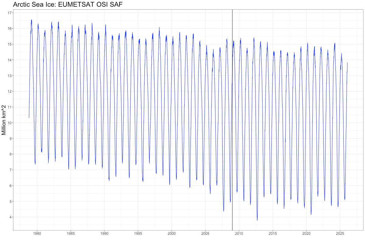
The vertical line is 2009, which is, amusingly, when one of our greatest politicians, John Kerry, said that “in five years” we’d have “the first ice-free Arctic.” Which only goes to prove what you already know. Politicians are not great friends to truth.
The average is about 11.4 million square km. But notice the huge swings each year. A lot of ice grows and melts. Such is the nature of weather. Standing in 2009, how could you have predicted no ice by 2014? Only if you were in the grip of powerful Theory. Or worse.
Anyway, by many definitions of “trend”, the ice from when satellites first launched and peered down upon us was somewhat decreasing. Not always, and not so much lately. This period, as far as relative ages go, is tiny. It is blazingly obvious there is a seasonal signal in the data. Most remember, alas Kerry did not, that winters are cold. As I write this, I can walk from my house in lower Michigan all the way to the UP on solid ice on Lake Michigan. This is because it was cold this winter, and for a long time. These things happen.
Unfortunately, this picture doesn’t show there are some missing observations. Out of the 17,267 available, 157 didn’t make it. Satellites aren’t perfect. Since the dots are all connected, we can see where here. It’s important, though, because in many, many, oh, a great many, software packages, one needs complete data. Or they break. They will not work. Sad, ain’t it.
It’s good to remember, though, because you have to cheat some way to overcome this. Not just you, but everybody. You’ll see words like “imputation” used. It means “Make the missing data up”. Which is fine in it’s way, as long as you keep the uncertainty you’ve added by making the data up. Which, as you will have seen coming, most do not. Over-certainty results.
I’m using a “Bayesian” time series package (all the code is below), but there are many options. All will given slightly different results. But that doesn’t matter to us, because we recall probability is the thing we want conditioned on all the information we have, which includes the analysis method and code.
They have a function called “auto.sarima” you’re welcome to try on this data. Stands for seasonal autoregressive integrated moving average. Review last week if you don’t remember what these are. We can see the obvious seasonality, and know its physical causes. There’s something of a trend, so the integrated part makes sense. The AR and MA points we’ll come to. The idea is it uses various magic, like the AIC and BIC things we didn’t discuss, to pick “optimal” values for all model parameters.
You can only run it after the “imputation”. Doesn’t work with missing values. Even so, it ran for about a hour on my fairly decent laptop, then crashed. Problem with all these Bayesian simulation methods is they are computer intensive, and they lack style and grace. We covered long ago why things like MCMC aren’t what they seem. Review them here.
Most of these methods will crash with data this big. Which isn’t real big, but big enough with MCMC.
So instead of opting for “optimal”, we’ll figure what works ourselves.
The sinusoidal signal is so obvious that we’ll fit a simple sine + cosine to it, along with a trend. The period is also given to us by the nature of the day, namely daily, or a 365-day cycle. We don’t “estimate” this using any kind of Fourier or spectral analysis, because we know what it is, and know that it’s related to a well known cause. (Well, maybe. At a college earth day in 1991, I surveyed students, and about half said the sun goes around the earth. But they cared about Saving the Planet.)
Here’s the model (blue) over the data (black). The missing data is now obvious.
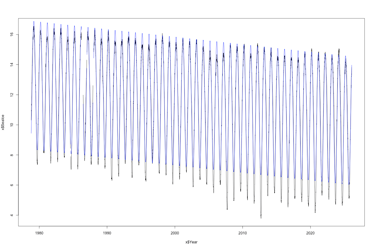
I didn’t make this as pretty, but you get the idea. The model gets the frequency right, but fails pretty badly at nailing the peaks: overshoots the highs and badly under predicts the lows. So there is lack of symmetry.
We’re not done. Next step is to look at the “residuals”, the data minus the model, which gives this:
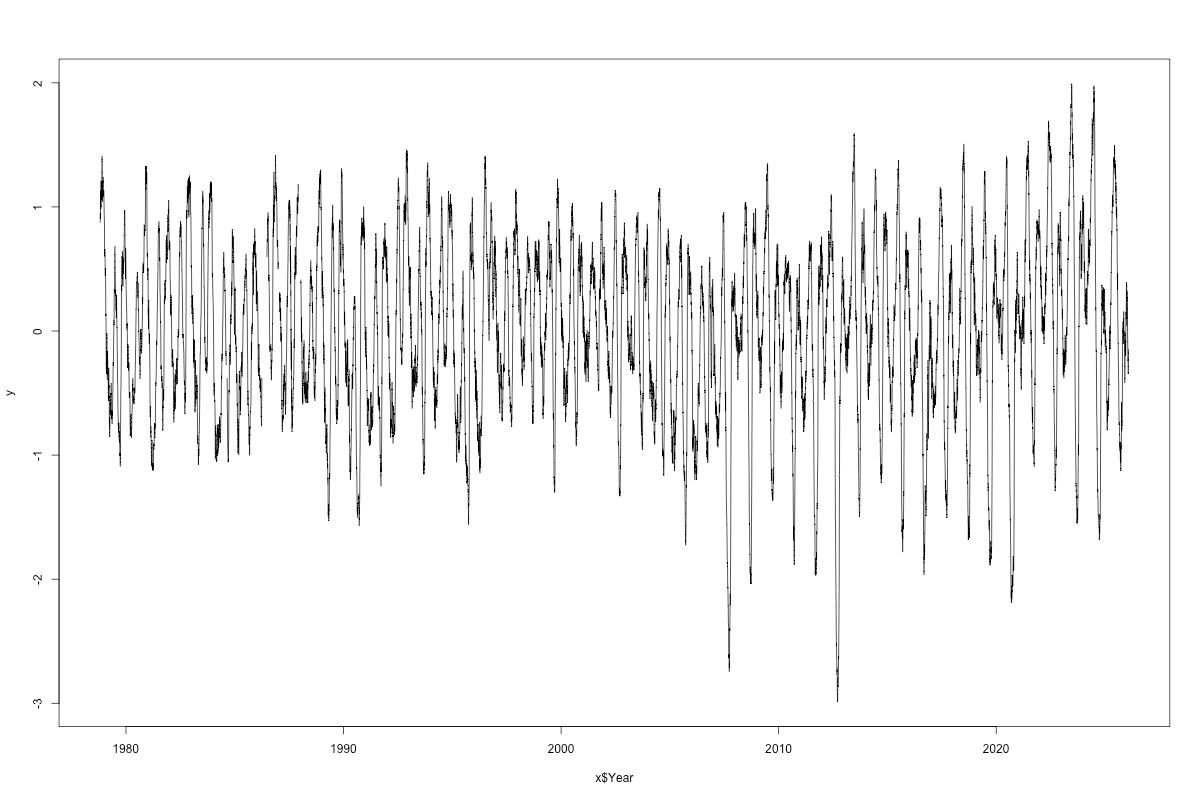
There’s any number of things that can be tried. We could have built in an asymmetry to the seasonal cycle, or we can work with these “residuals” in the ordinary time series way. For instance, by looking at auto and partial auto-correlations, which give us the p and q we learned last week. But only because hypothesis testing, which is weak sauce. There is no correct answer here. Because it’s all just correlations.
The causal part we got close to with the seasonality, but there still may be useful correlations in this data we can squeeze some information out of.
In order to use these ad hoc tools we need to fill in the missing data, by guessing (we didn’t need to do it for the sine+cosine, which was just a regression). We’ll use the predictions from the seasonal model and hope for the best. We ought to keep track of the uncertainty added by this maneuver. I’m going to ignore it here, so that everything is typical. How? By “redoing” our final answer for each of the possible numbers we impute, and weight the whole by the probability of the imputations. That’s too much to do for this introductory example, and anyway there is not much missing data.
Anyway, once we have complete data, we can do the acf and pacf:
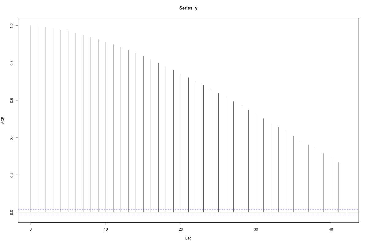
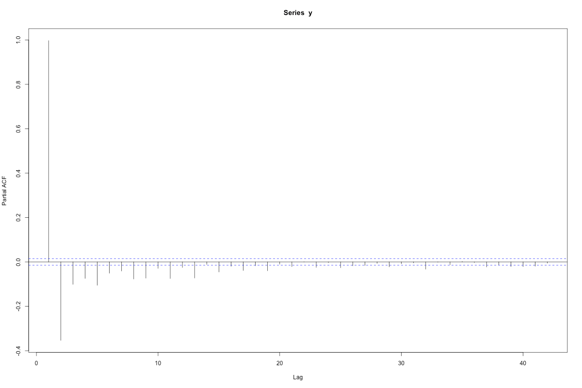
When you see lines sticking out beyond the magic bounds, given by wee p-value like calculations, you’re supposed to say there are “significant” correlations. Here, a strong negative first partial correlation, and a lot of correlation in the mean term (the acf part).
Now we can do this by hand, or we can use the “optimal” algorithm. That algorithm broke when we used it on the raw data, and not just because it had missing values. The seasonal signal allowed too many possibilities, too many things to check. Since we’re just doing it on the residuals, we can get away with it.
The algorithm gave us—after the seasonality model was first removed, remember—an ARMA(2,2) model for the residuals. The two p’s were 0.995 and -0.0005; the two q’s were 0.317 and 0.143. But these are NOT REAL, you must always understand. They are merely parameters in a model, and we ought to “integrate them out” of any resulting prediction. Else our prediction, just using these values as if they were real, will be too certain. Which is, of course, what most do.
But we can do it, because this package includes a method to do predictive posteriors (rare). Here is the 80% predictive window for the residuals (there is no reason in the world to use a 95% window). These are not “confidence” or “credible” intervals. These give the 80% chance the residual will appear in the window on the given day. Pure probability.
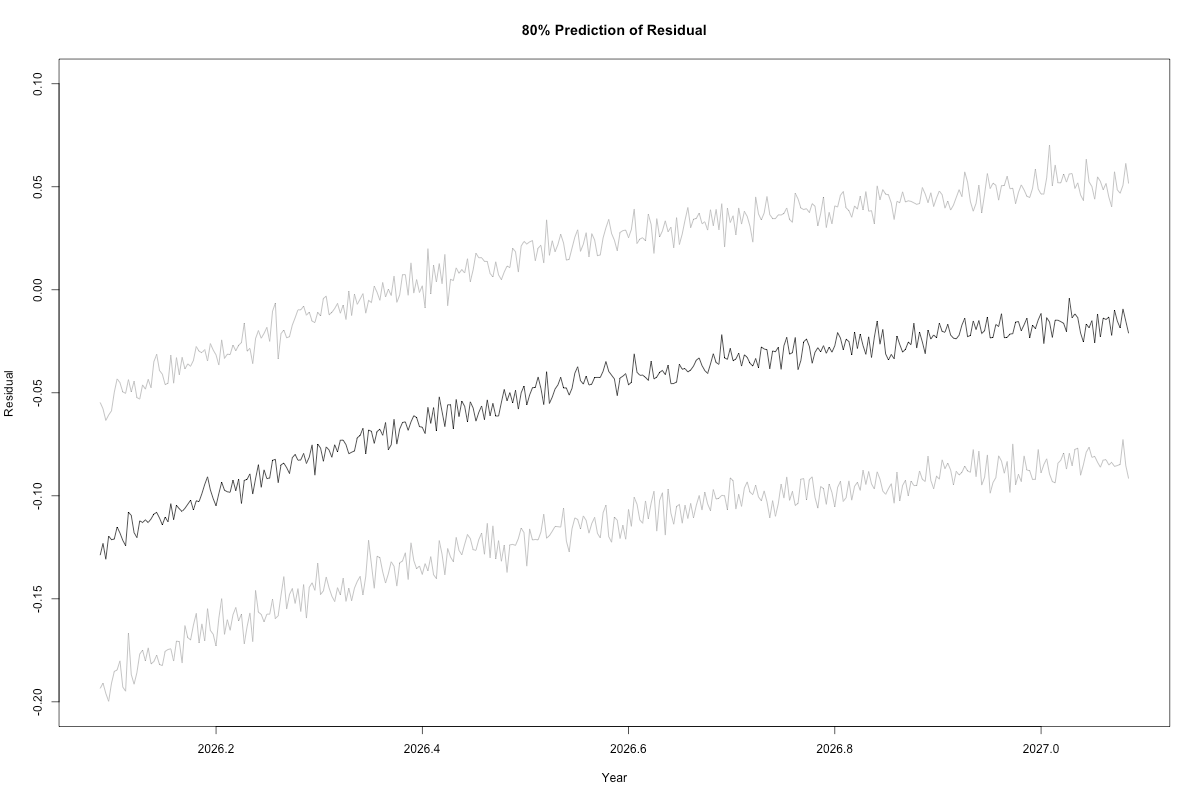
Carry it out long enough and the model gravitates to 0, which is just (of course) the mean. This model has limited scope. All models do.
We need to add back the seasonality, with its own predictive uncertainty (I was lazy here and just used the lm function’s predictive uncertainty, which is close enough to the Bayesian for our purposes):
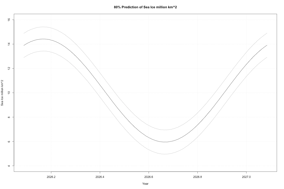
Remember our seasonality model stank up the place with its lows. So this predicted low might be too high. On the other hand, it’s been a mighty cold year, but our model didn’t see that. It would have only got lucky.
“But Briggs, here’s a list of 12 things where I think you went wrong, and what I would have done differently.”
Only 12? And I didn’t go wrong anyway. This is all just correlations. I have zero doubt you have a way to better use them and get tighter predictions. But that doesn’t make mine wrong, just less good. That’s the problem with time series. Endless bickering.
The keys are this: use whatever causality you can, and remember the rest is just correlations, which may or may not work, and state everything in terms of actual probability of real observables. No parameters, no hypothesis testing. We haven’t verified this model, but could. Simply wait a year and come back to it.
Next week I might stress the causality angle. I don’t want us to learn methods. There are endless methods. I want us to understand.
Here are the various ways to support this work:
Subscribe at Substack (paid or free)
Cash App: $WilliamMBriggs
Zelle: use email: matt@wmbriggs.com
Hire me
PASS POSTS ON TO OTHERS
# R code
# It may or may not work. No gurantees
# https://osisaf-hl.met.no/v2p3-sea-ice-index
#   ftp://osisaf.met.no/prod_test/ice/index/v2p3/nh/osiaf_nh_sie_daily.txt
# sea ice extent, northern hemisphere
# FracYear YYYY MM DD SIE[km^2]
# Area: Northern Hemisphere
# Quantity: Sea Ice Extent
# Product: EUMETSAT OSI SAF Sea Ice Index v2p3 (demonstration)
# References: Product User Manual for OSI-420, Lavergne et al., v1.2, 2023
# Source: EUMETSAT OSI SAF Sea Ice Concentration Climate Data Records v3 data, with R&D input from ESA CCI (Lavergne et al., 2019)
# Creation date: 2026-02-02 10:01:24.578948

# I renamed the long ugly file "d.txt" because I am lazy

# Read in and eliminate all distractions
x = read.table('d.txt',header=TRUE,sep=' ')
   i = which(x$SeaIce < 0)
  x[i,] = NA
  #x = x[-i,]
  x = x[,c(1,5)]
  x$SeaIce = x$SeaIce/1e6
  summary(x)

# Plot
g=ggplot(data = x, aes(x = Year,y=SeaIce)) +
   geom_line(linewidth=.5, color='blue')+
   scale_y_continuous(breaks = scales::pretty_breaks(n = 12),labels = scales::comma)+
   scale_x_continuous(breaks = scales::pretty_breaks(n = 12))+
   geom_vline(xintercept = 2009) +
   theme_bw()+
  labs(title = "Arctic Sea Ice: EUMETSAT OSI SAF ",
       x = "",
       y = "Million km^2")+
              theme(axis.text.x = element_text(size = 12),
             axis.text.y = element_text(size = 12),
             axis.title.x = element_text(size = 18),
             axis.title.y = element_text(size = 18),
             plot.title = element_text(size=22))

g

# Simple sine+cosine + trend model
per=365 # time period
t = 1:length(x$SeaIce)
xc  = cos(2*pi/per*t)
xs  = sin(2*pi/per*t)
fit <- lm(SeaIce ~ t  + xc+ xs, data=x)

pred <- predict(fit, newdata=data.frame(t=t,xc = xc,xs=xs))
plot(x$Year,x$SeaIce,type='l')
  lines(x$Year, pred, col="blue")

# Residuals & Imputation
y = x$SeaIce - pred
i = which(is.na(x$SeaIce))
w = x$SeaIce
w[i] = pred[i]
y = w - pred

# ACF and PACF
acf(y)
pacf(y)

# Residual time series model and plot with 80% predictive interval
fit = auto.sarima(y,iter = 500,chains = 1)

fc = posterior_predict(fit,h=365)
  Y = tail(x$Year,1)+(1:365)/365
  plot(Y,apply(fc,2,median),type='l',xlab='Year',ylab='Residual',ylim=c(-.2,.1),main='80% Prediction of Residual')
    lines(Y,apply(fc,2,quantile,probs=.9),lwd=.5,col="#555555")
    lines(Y,apply(fc,2,quantile,probs=.1),lwd=.5,col="#555555")

# The Final model, adding in the sin+cos and residual model with 80% predictive interval
per=365
t = 1:length(x$SeaIce)
xc  = cos(2*pi/per*t)
xs  = sin(2*pi/per*t)
fits <- lm(SeaIce ~ t  + xc+ xs, data=x)

t = (length(x$SeaIce)+1):(length(x$SeaIce)+365)
xc  = cos(2*pi/per*t)
xs  = sin(2*pi/per*t)
pred <- predict(fits, newdata=data.frame(t=t,xc = xc,xs=xs),interval = "prediction", level = 0.8)
 pred = as.data.frame(pred)

  plot(Y,apply(fc,2,median)+pred$fit,type='l',xlab='Year',ylab='Sea Ice million km^2',ylim=c(4,16),main='80% Prediction of Sea Ice million km^2')
    lines(Y,apply(fc,2,quantile,probs=.9)+pred$upr,lwd=.5,col="#555555")
    lines(Y,apply(fc,2,quantile,probs=.1)+pred$lwr,lwd=.5,col="#555555")
    grid()
I don't understand it, but I love it.
Which also kind of encapsulates my view of women, which I also love but will never understand.
No offense intended but I don't get it. Why go to all the extreme effort to make a model? One which doesn't fit? Why not just USE THE DATA to predict the future? Eyeball it. Zero residuals. No sweat.
Also, who the ef cares about Arctic sea ice? Why is that a thing? Who made it a thing? I think if you bore into those questions you'll find at the bottom elite billionaires who rape (and sometimes eat) children. Total depraved sickos who use their obscene wealth to harm the innocent for fun.
There are time series that matter. How fast is the river rising? When will it hit flood stage? Or, how many children are probably going to be raped next week by princes, bankers, and other perverted elites? What's the current Satanic Quotient and how has it been trending over the last century? Sea ice is utterly inconsequential.