How Predictive Statistics Can Help Alleviate, But Not Eliminate, The Reproducibility Crisis

Predictive statistics can help alleviate the Reproducibility Crisis by, in a word, eliminating p-values. And replacing them with superior measures more useful in quantifing the uncertainty present.

Below is some, what I hope is, clear R code (not optimized or prettified in any way) to demonstrate what I mean. Try it yourself for fun.

Step 1. Make up n numbers, x and y, that have nothing to do with one another.

Step 2. Do a regression of y and x.

Step 3. Calculate the p-value and "effect size". These should show "no effect", i.e. p > magic number 95% of the time and size = 0, because no effect exists. All agree with this.

Step 3. Compute this probability:

     Pr = Pr(y at x+1 > y at x | our assumptions, data).

Since there is no effect, the probability that y at a value of x one unit is higher than a y at x should by 50%, conditional on the belief no effect exists and we're just making up numbers. Any difference between 50% and Pr is an indication of the "strength" of the predictive (not causal!) relationship between x and y. If you don't understand Step 3, study it until you do.

In regression, the effect size is the amount, on average, that y changes given a unit increase in x. This is the theory. If y and x have nothing to do with one another, the effect size should be 0. Y should not change, on average, with x.

Same thing predictively. The probability of y when x is (say) 8 being greater than y when x is 7 should be 50%, because x provides no information about y. If you are picking numbers from a "normal", or any "distribution", the chance the second one is larger than the first is 50%.

Obviously, as I have emphasized countless times, p-values exaggerate evidence. Everybody, without exception, even those who say they don't, takes them to indicate the strength of the relationship between x and y.

The p-value means only this: the probability the statistic inside the regression would be larger in absolute value than it actually is assuming there is no information in x about y, and if you repeated the experiment that gave rise to the data an infinite (not small) number of times. Useless information.

The predictive probability is what you want to know in plain English. "Say, what's the chance y gets bigger (or smaller) when x increases?" That's why you did the regression in the first place! That's exactly what the "effect size" and p-value cannot and do not tell you. But the predictive probability can and does.

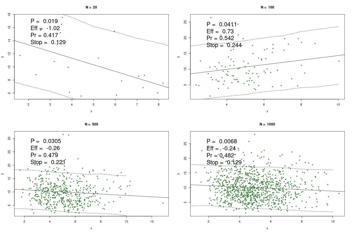
Here's one example of making up some numbers, using different sizes, n = 20, 100, 500, and 1000. Way it works is we keep making up x and y until the regression throws a wee p, which is the point researchers would stop and yell "WhooPee!" Wee p's are notoriously easy to generate, just by twiddling the data, changing the statistic, increasing n, and so on.

Thus we're trying to simulate the "research process", which may be characterized as the Hunt For Wee Ps. Remember: there is nothing in x that says anything about y. But we can still get a wee p with ease.

The P is the p-value, Eff is the effect size (which should = 0), Pr is the predictive probability above, and, for fun, Stop is the negative binomial probability (dnbinom(1,k,0.95); which if you know, you know; if not, it's a measure of how long it took to get the wee p at these conditions).

The solid line is, of course, the regression. The dashed lines are the 90% (not 95%) predictive intervals. I.e. at any x, there is a 90% chance y would be within this interval, conditional on the data, model, etc.

Now you can play with this, but it's well known that with smaller samples we get more variability. Thus the largest effect size in this simulation is with n = 20. The p's are all publishable, and would confirm your theory that x causes y.

Every researcher would give at least solid hints that x causes y. That's a story for another day.

Contrast the p's with the Pr's. These should be 0.5, but they're slightly different. When n = 20, we see the largest departure from 50%. Again, greater variability.

Point is this: which regression-driven headline sounds less exciting? "X linked to Y, p < 0.02", or "There is a 42% chance Y will decrease when X increases by 1"?

Try it for n = 1000: "X linked to Y, p < 0.007", or "There is a 48% chance Y will decrease when X increases by 1"?

Well, you get the idea, I hope. The predictive probability can still lie to you. Look, when you're doing your experiment, you only have what you have in front of you. The temptation to tweak and fiddle with data is too overwhelming, and you, too, will be overwhelmed. But you can't make nothing sound as good using full uncertainty as you can with p-values. P-values exaggerate.

You can always make nothing sound like something. There is no procedure in the world that can ever change that. At least the predictive approach, beyond producing answers in plain English, makes it more difficult to fool yourself---and others. It also allows your model to be tested by anybody, which p-values don't and can't.

Subscribe or donate to support this site and its wholly independent host using credit card or PayPal click here

Update Answering some critics on Twitter, who think p-values are saved because this simulation demonstrates selection bias. Dudes. This piece which is ABOUT selection bias. It assumes the bias, which I called the "research process". It then shows two measures, the p-value and the predictive. Both suffer from the (on purpose!) bias. But the predictive gives less certainty, as it always does even when selection bias does not exist.

P-values always exaggerate evidence and tell you what you don't want to know. Predictive probs give you answers in plain English (or even Dutch!).

CODE

library(rstanarm)
png('predictive.png',width=1200,height=800)
par(mfrow=c(2,2))
n = c(20,100,500,1000)
for(j in 1:4){
p = 1
k = 0
while(p>0.05){
  k = k + 1
  x = rgamma(n[j],10,2) # most real-life data is non-negative and more like this 
  y = rgamma(n[j],5,.5) # than normal. but feel free to change to others and see
                        # what it does
  fit = glm(y~x)
  p = summary(fit)$coefficients[2,4]
}
eff = summary(fit)$coefficients[2,1]
k
negb = dnbinom(1,k,.95)
w = data.frame(x=x, y =y)  # rstan likes to have data frames
z = data.frame(x = seq(0,10,1))
fit.s = stan_glm(y~x,data=w)
    pr = posterior_predict(fit.s, newdata=z) # predictive probs
    z$m = colMeans(pr)
    z$lo = apply(pr, 2, quantile, probs=.05)
    z$hi = apply(pr, 2, quantile, probs=.95)
# this is only quick and dirty and, i hope, readable
# any plain language question you have about model can be
# answered like this
a = 0
m = dim(z)[1]
for(i in 2:m){
  a = a+sum(pr[,pr[,i-1])/4000 # default number in pr
}
Pr = a/(m-1)
  
plot(x,y,main=paste('N = ', n[j]),col="#448844", pch=20)
  abline(fit)
  lines(z$x,z$lo,lty=2)
  lines(z$x,z$hi,lty=2)
  legend(min(w$x),1.1*max(w$y),
         paste('P = ',round(p,4),
               '\nEff = ', round(eff,2),
               '\nPr =', round(Pr,3),
               '\nStop = ',round(negb,3)), bty='n' ,cex=2)
}  
dev.off()
Subscribe or donate to support this site and its wholly independent host using credit card or PayPal click here
]]>